Chapter 2 The Methodology
2.1 Setting up
We consider the fundamental problem of making inference about an unknown function f that predicts an output Y using a \(p\)-dimensional vector of inputs \(x = (x_1, ..., x_p)\) when \[Y = f(x) + \epsilon, \text{with } \epsilon \sim N(0, σ^2).\]
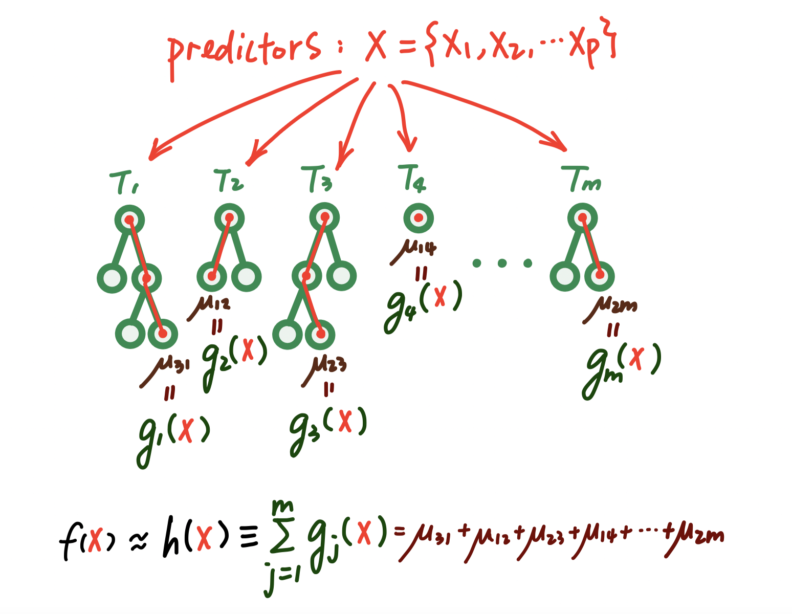
To do this, we consider modeling or at least approximating \(f(x) = E(Y | x)\), the mean of \(Y\) given \(x\), by a sum of \(m\) regression trees \[f(x) \approx h(x) ≡ \sum_{j=1}^m g_j(x), \] where each \(g_j\) denotes the mapping function associated with the \(j_{th}\) tree.

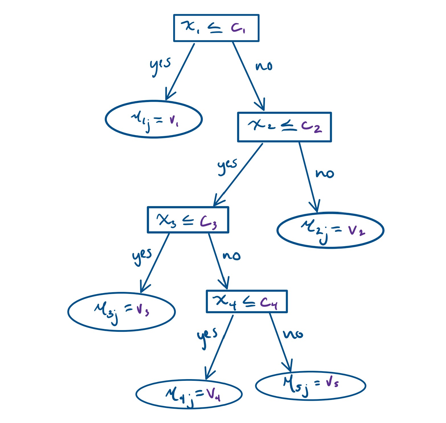
Figure 2.1: A visual representation of \(g(x;T_j, M_j)\) . Square boxes represent the splitting rules, while circles denote the terminal nodes.
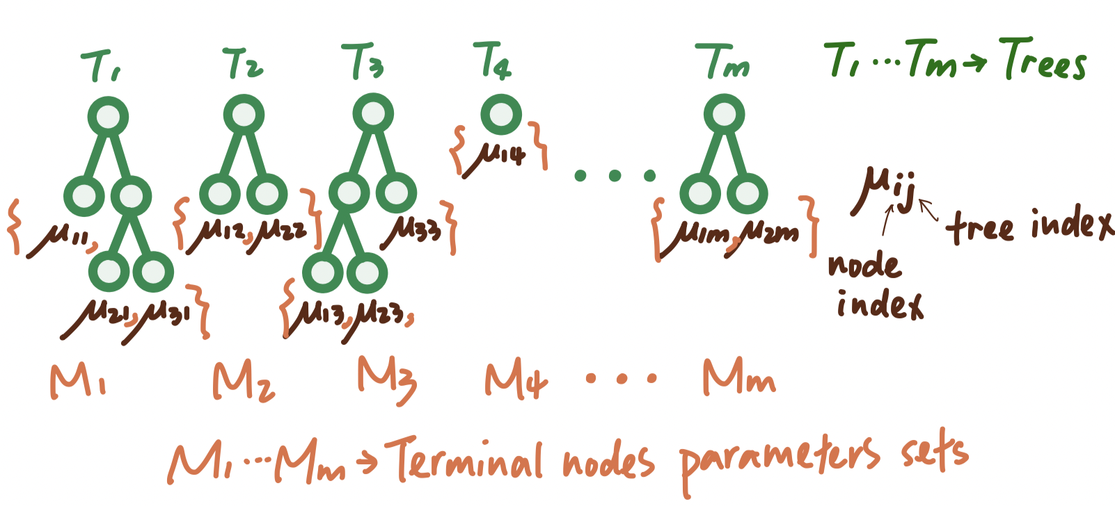
Getting into more details, let \(T\) denote the set of all binary regression trees, and a full list of \(m\) trees can be denoted as the set \(T = \{T_1, T_2, T_3, ...\}\) For a specific binary regression tree \(T_j\) that has \(b\) terminal nodes, let \(M_j = \{\mu_{1j}, \mu_{2j}, \mu_{3j}, ..., \mu_{bj}\}\) denote the parameters for those \(b\) terminal nodes of this tree \(T_j.\) Under this setting, \[ \begin{align*} Y & = \sum^{m}_{j = 1} g_j(x) + \epsilon\\ & = \sum^{m}_{j = 1} g(x; T_j, M_j) + \epsilon \end{align*} \] where \(g(x; T_j, M_j)\) is a function that assigns \(\mu_{ij}\in M_j\) to \(x\). The expected value of the output \(Y\) given \(x\), \(E(Y | x)\), is the sum of all the \(\mu_{ij}\) values assigned to \(x\) by the functions \(g(x; T_j, M_j)\). When there are multiple trees (\(m > 1\)), each \(\mu_{ij}\) contributes only a part of \(E(Y | x)\), which is different from a single tree model. Each \(\mu_{ij}\) represents a “main effect” if \(g(x; T_j, M_j)\) depends on only one component of \(x\) (a single variable), and an interaction effect if it depends on more than one component (more than one variable).

Figure 2.2: A visual representation of the set-up of a sum-of-tree model.

Figure 2.3: A visual representation of the prediction process of a sum-of-tree model.
Therefore, the sum-of-trees model can capture both main effects and interaction effects, with interaction effects of varying orders depending on the sizes of the trees. In the special case where every terminal node assignment depends on just a single component of \(x\), the sum-of-trees model simplifies to a simple additive model. Let \(m\) denote the number of trees we will build in a sum-of-trees model. For a fixed \(m\) , a sum of tree model is determined by \(T = \{T_1, T_2, T_3, ...,T_m\}\), \(M = \{M_1, M_2, M_3, ..., M_m\}\), and \(\sigma\). Thus, all the priors that we need in this setting would be: priors over \((T_1, M_1), (T_2, M_2), (T_3, M_3), ... (T_m, M_m)\) and the prior over \(\sigma\). For all those priors, we have their joint probability function as: \[ \begin{align*} & P((T_1, M_1), (T_2, M_2), (T_3, M_3), ... (T_m, M_m), \sigma) \\ & = \prod^{m}_{j=1} (T_j, M_j)P(\sigma) \;\; \text{by assumption of iid trees}\\ & = [\prod^{m}_{j=1} P(M_j|T_j)P(T_j)]P(\sigma)\;\; \text{law of total probability} \\ & = [\prod^{m}_{j=1} P(\mu_{1j}|T_{j})P(\mu_{2j}|T_{j})...P(\mu_{bj}|T_{j})]P(\sigma) \\ & = [\prod^{m}_{j=1} \prod^{b_j}_{i=1} P(\mu_{ij}|T_j)P(T_j)]P(\sigma) \;\; \text{iid parameters of terminal nodes in a specific tree}\end{align*}\] Thus, after those calculation, we figured that there are only \(4\) priors that we need to think about, which are \(T_j, \mu_{ij}|T_j\), \(\sigma\) and \(m\). We will talk about them one by one in the next section.
2.2 Prior models and tuning
2.2.1 The \(T_j\) Prior
This prior defines how the decision trees in the model are built, specifically how they make splits at each non-terminal node.
The prior of \(T_j\) is specified by the three below aspects.
Depth-based stopping: The deeper a node in the tree, the less likely it is to continue branching. This is controlled by manipulating the probability that a node at depth \(d\) (= 0, 1, 2, …) is nonterminal. Specifically, parameters \(\alpha\) and \(\beta\) are controlling this probability, where \(\alpha\) affects the initial likelihood of branching and \(\beta\) controls how quickly this likelihood decreases as the tree gets deeper.
\[ P(\text{node of depth d is nonterminal}) = \alpha(1 + d)^{-\beta} \text{ where } \alpha \in (0, 1), \beta \in [0, \infty) \]
In order to keep the \(m\) trees small so they can be summed, we can choose to use values \(\alpha = 0.95\) and \(\beta = 2\)
Variable selection: Each time the tree decides to split, it randomly chooses which variable (or feature) to split on. This choice is uniform, meaning every variable has an equal chance of being selected. This is controlled by setting the distribution on the splitting variable assignments at each interior node.
Splitting rule: For the chosen variable, the specific way it splits (i.e., the rule it uses to divide the data) is also chosen randomly. This is controlled by setting the distribution on the splitting rule assignment in each interior node, conditional on the splitting variable. The distribution on the splitting rule assignment in each interior node, conditional on the splitting variable
For quantitative variable \(x_q\), \[\text{splitting rule | variable } x_q \sim Unif(min(x_q), max(x_q))\] For categorical variable \(x_c\), each category has the same chance of being chosen.
All these prior settings about \(T_j\) help ensure that the trees remain small and manageable, which is important when they are combined to form the sum of trees model.
2.2.2 The \(\mu_{ij} | T_j\) prior
The \(\mu_{ij} | T_j\) prior uses the conjugate normal distribution:
\[ \mu_{ij} | T_j \sim N(\mu_\mu, \sigma_\mu^2) \]
The individual predictions \(\mu_{ij}\) ’s are assumed to be independent and identically distributed (apriori i.i.d.).
\[ E(Y|x) \sim N(m\mu_\mu, m\sigma_\mu^2), \]
where it is highly probable for \(E(Y|x)\) to fall between \(y_{min}\) and \(y_{max}\).
Because of this, we want to choose values of \(\mu_\mu\) and \(\sigma_\mu\) so that \(E(Y|x) \sim N(m\mu_\mu, m\sigma_\mu^2)\) is most plausible in the interval of (\(y_{min}\), \(y_{max}\)). We can do this by choosing values of \(\mu_\mu\) and \(\sigma_\mu\) so that:
\[ \begin{align*} m\mu_\mu - k \sqrt{m}\sigma_\mu & = y_{min} \\ m\mu_\mu + k \sqrt{m}\sigma_\mu & = y_{max} \end{align*} \]
From here, we can rescale \(Y\) so that our interval \((y_{min}, y_{max})\) is \((-0.5, 0.5)\) which gives
\[ \begin{align*} \mu_\mu & = 0 \\ \sigma_\mu & = \frac{0.5}{k\sqrt{m}} \end{align*} \]
The value \(k=2\) is a good default choice as this would yield a 95% prior probability that \(E(Y|x) \in (y_{min}, y_{max})\).
2.2.3 The \(\sigma\) prior
For \(\sigma^2\) we use the inverse chi-square distribution:
\[ \sigma^2 \sim \frac{\nu\lambda}{\chi^2_{\nu}} \]
For determining the hyperparameters \(\nu\) and \(\lambda\), we use the data-informed prior approach using a “rough data-based overestimate” of \(\hat{\sigma}\) for \(\sigma\).
We suggest setting \(\nu\) between 3 and 10 for favorable results, and \(\lambda\) as either 0.75, 0.90, or 0.99, ensuring that the \(q\)th quantile of the prior on \(\sigma\) matches \(\hat{\sigma}\), expressed as \(P(\sigma < \hat{\sigma}) = q\).
For simplicity, the default can be \((\nu, q) = (3, 0.9)\), which generally avoids extremes.
2.2.4 Choosing m
Recalling from earlier, \(m\) represents the number of trees in our BART model.
To select an optimal \(m\), people often use cross-validation (CV), but this process can be time-consuming.
An alternative to CV is to default to \(m = 200\), as the algorithm’s predictive performance significantly improves from \(m = 1\) to around 200 trees. However, excessively large \(m\) values can lead to a gradual degradation in BART’s performance.
2.3 Backfitting with MCMC Algorithm
2.3.1 Algorithm set-up
Hastie and Tibshirani (2000) considered a similar application of the Gibbs sampler for posterior sampling for additive and generalized additive models with σ fixed, and showed how it was a stochastic generalization of the backfitting algorithm for such models. For this reason, Chipman et al. (2010) refer to their algorithm as backfitting MCMC.
Given the observed data \(y\) and unknown parameters \((T_1, M_1), ..., (T_m, M_m)\) and \(\sigma\), the posterior distribution of these parameters can be represented as \[p((T_1, M_1), ..., (T_m, M_m), \sigma|y),\]which determine the sum-of-trees model.
Generally speaking, this backfitting algorithm iteratively updates each parameter in \((T_1, M_1), ...(T_m, M_m)\) and \(\sigma\) using the most current knowledge of the other parameters, which is just the idea of Gibbs sampler.
Specifically, let \(T_{(j)}\) represent all trees except \(T_j\), and let \(M_{(j)}\) represent all terminal nodes parameters except \(M_j\). In this Gibbs sampler, we loop from \(j = 1\) to \(j = m\) to draw \((T_j, M_j)\) given \((T_{(j)}, M_{(j)}), \sigma, y\). That is, \[(T_j, M_j) |T_{(j)}, M_{(j)}, \sigma, y\] We also need to update \(\sigma\) based on the most recent knowledge of \((T_1, M_1), ...(T_m, M_m)\): \[\sigma|T_1,...T_m, M_1, ...M_m, y\]
The posterior distribution \(p(T_j, M_j|T_{(j)}, M_{(j)}, \sigma, y)\) depends on four things \(T_{(j)}, M_{(j)}, \sigma, y\). But it depends on three of them \(T_{(j)}, M_{(j)}, y\) only through \[R_j \equiv y-\sum_{k\neq j}g(x;T_k, M_k),\]which is an \(n\)-vector where the \(j_{th}\) entry records the residuals between the real value and the current estimate, where the current estimate is just the sum of the partial results gotten from all but the \(j_{th}\) trees.
Consequently, drawing \((T_j, M_j)\) given \(T_{(j)}, M_{(j)}, \sigma, y\) can be regarded as equivalent to drawing from \(R_j, \sigma\), expressed as: \[(T_j, M_j)|R_j, \sigma\]
Here, \(R_j\) can be understood as the target value that the single tree model \(T_j\) aims to get at, essentially acting as the “data” for this purpose. Formally, \[R_j = g(x;T_j, M_j)+\epsilon.\]
The calculation for \(p(T_j|R_j, \sigma)\) is detailed as follows: \[ \begin{align*} p(T_j|R_j, \sigma) &= p(T_j)p(R_j|T_j,\sigma) \\ &\propto p(T_j)\int p(R_j,M_j|T_j,\sigma)dM_j \\ &= p(T_j)\int p(R_j|M_j, T_j,\sigma)p(M_j|T_j, \sigma)dM_j \end{align*} \]
Given the use of a conjugate prior for \(M_j\), we can derive \(p(T_j|R_j, \sigma)\) in a closed form up to a normalization constant.
In summary, the whole backfitting algorithm utilizing the idea of Gibbs sampler is to successively draw \(T_1, M_1, ..., T_m, M_m, \sigma\) in each full iteration. Thus, each interation is consists of \(2m+1\) steps:
\[ \begin{align*} T_j & |R_j, \sigma\\ M_j & |T_j, R_j, \sigma \\ \sigma & |T_1, M_1,...T_m, M_m,y, \sigma \end{align*} \]
Tree drawings \(T_j\) are facilitated using the Metropolis-Hastings algorithm, which proposes new tree configurations based on the current tree through 4 modifications: growing a terminal node, pruning a pair of terminal nodes, changing a nonterminal rule, and swapping rules between parent and child nodes, with associated probabilities of 0.25, 0.25, 0.40, and 0.10 respectively.
Subsequently, \(M_j\) is drawn independently for the terminal nodes \(\mu_{ij}\) from a normal distribution, facilitating the calculation of the next residual \(R_{j+1}\), which is crucial for the upcoming draw of \(T_{j+1}\).
2.3.2 Posterior inference statistics
Every output from the algorithm can be used to build a tree-based model. Summing up all the tree outputs from each draw (indexed by \(j\)), we get a sequence of models that gradually approach the true underlying model, \(f(·)\). This is noted as: \[ f^*(·) = \sum_{j=1}^m g(·; T^*_j, M^*_j) \]
By running the algorithm for a sufficient number of iterations, especially after a preliminary ‘burn-in’ period, the sequence of \(f^{∗}\) draws (like \(f^{∗}_1\), \(f^{∗}_2\), …, \(f^{∗}_K\)) gives a good approximation of the posterior distribution of the true model \(f(·)\).
These tree-based model outputs can be used to estimate various statistical measures, like the mean or median of \(f(·)\), by averaging or finding the median of the post-burn-in samples.
To predict values or behaviors (\(Y\)) at a new or existing data point (\(x\)), you can use the average or median of these post-burn-in tree models. To understand the reliability of these predictions at different values of \(x\), you look at how much the predictions vary among these models. This can be captured by calculating intervals (quantiles) around the predictions. By observing which variables are most frequently used in the models (especially as the number of trees \(m\) is reduced), BART helps identify the most important predictors for the response variable \(Y\). This process is effectively a competition among predictors to demonstrate their relevance to the model.
2.3.3 Conclusion
In summary, the backfitting MCMC algorithm generates multiple potential
models by simulating how trees would split based on data. These models
converge over many iterations to a true model. By analyzing these
models, one can make predictions, assess uncertainty, understand
variable importance, and determine the impact of specific predictors on
the outcome.
2.4 BART Probit for Classification
We have discussed BART model for continuous \(Y\), but BART can also be used for binary outcome \(Y\; (= 0\text{ or }1)\).
2.4.1 What is Probit/Probit Model?
A probit model is a type of regression where the dependent variable \(Y\) can take only two values, for example married or not married, similar to logistic regression. However, probit model has different distribution than logistic regression. Specifically, we assume that the model takes the form \[P(Y = 1 \mid X) = \Phi(X^\text{T} \beta)\] where \(P\) is the probability and \(\Phi\) is the cumulative distribution function (CDF) of the standard normal distribution \(N(0,1)\).
2.4.2 Setup BART for Classification
Thus, BART model extends to be \[p(x) \equiv P [Y = 1 \mid x] = \Phi[G(x)]\] where \[G(x) \equiv \sum_{j=1}^{m} g(x; T_j, M_j),\] our sum of regression trees.
2.4.3 Modification of Regularization Priors
BART extension to binary outcome requires imposing a regularization prior on \(G(x)\) and implementing a Bayesian backfitting algorithm for posterior computation. Fortunately, these can be obtained with only minor modifications of the methods for continuous \(Y\). Since we use probit model distribution, we implicitly assume \(\sigma = 1\) and so only a prior on \((T_1, M_1), \ldots, (T_m, M_m)\) is needed. Proceeding exactly as BART for continuous \(Y\), we consider a prior of the form: \[ p((T_1,M_1),\ldots,(T_m,M_m)) = \prod_j \left[ p(T_j) \prod_i p(\mu_{ij}|T_j) \right] \] where each tree prior \(p(T_j)\) is the same as tree prior for continuous \(Y\). So we need to figure out the updated prior on \(p(\mu_{ij}|T_j)\). We choose \(p(\mu_{ij}|T_j)\) to cover most of the relevant \(p(x)\) values by considering the interval \((\Phi[-3.0], \Phi[3.0])\), which is often practical. Following the motivation of \(\mu_{ij}\) when having continuous \(Y\), we recommend the choice: \[ \mu_{ij} \sim N \left(0, \sigma_{\mu}^2 \right) \] where \(\sigma_{\mu} = \frac{3.0}{k\sqrt{m}}\), and \(k\) is chosen such that \(G(x)\) will likely fall within the interval \((-3.0, 3.0)\). Therefore, this prior can also limit the effect of the individual tree components of \(G(x)\) as \(\mu_{ij}\) is shrinking towards zero. Thus, every small tree is a weak learner. As \(k\) and/or the number of trees \(m\) is increased, this prior will become tighter, leading to greater shrinkage applied to the \(\mu_{ij}\). When choosing \(k\), statisticians found that values between 1 and 3 work well and they suggest using \(k = 2\) as the default choice, or determine it through cross-validation.